A Little Celebration of Excel Simplicity - COUNTIF(S)
- Rachel | The Blue Star Academy
- Jan 23, 2022
- 3 min read
Updated: Feb 10, 2022
The humble COUNTIF(S) function is the topic of today’s blog post, but before you roll your eyes and click away, hear me out! I’ve got a cool idea on how you can maximise your use of this handy little calculation.
When I first sat down to ‘formally’ learn Microsoft Excel, the COUNTIF(S) function was the one I got my head around first and it was quite a bittersweet experience. Prior to that very first enlightening =COUNTIF moment, I’d been manually adding up the various bits of information on my spreadsheets, assuming that what I was doing was what everyone else did.
In learning this function, I simultaneously felt horror at the many hours I had wasted, but also elation that I had somehow uncovered one of Microsoft Excel’s closely guarded secrets and now I was all-powerful!
So, yes. The COUNTIF(S) function is quite humble and chances are you are far more advanced in your Excel knowledge than I was all those years ago, it’s existence hasn’t passed you by and it’s a lovely little go-to tool in your Microsoft Excel toolkit.
If not, you can familiarise yourself using the Function Directory on my FREE membership site. Here’s the link for COUNTIF and for COUNTIFS
But this post is my attempt to celebrate the COUNTIF(S) function since it will always have a special place in my heart. It’s the very first eureka moment myself and Microsoft Excel shared and the true starting point on my personal learning journey.
Without further ado, here is an idea on how you can use a COUNTIF(S) function in a way you perhaps have not considered before!
Using COUNTIFS to Review Data that Matches a Specified Date Range
First up, let’s imagine we have a set of data that looks something like this:

We want to report on this data by month. All the options are there to enable this so it should be fairly straightforward.
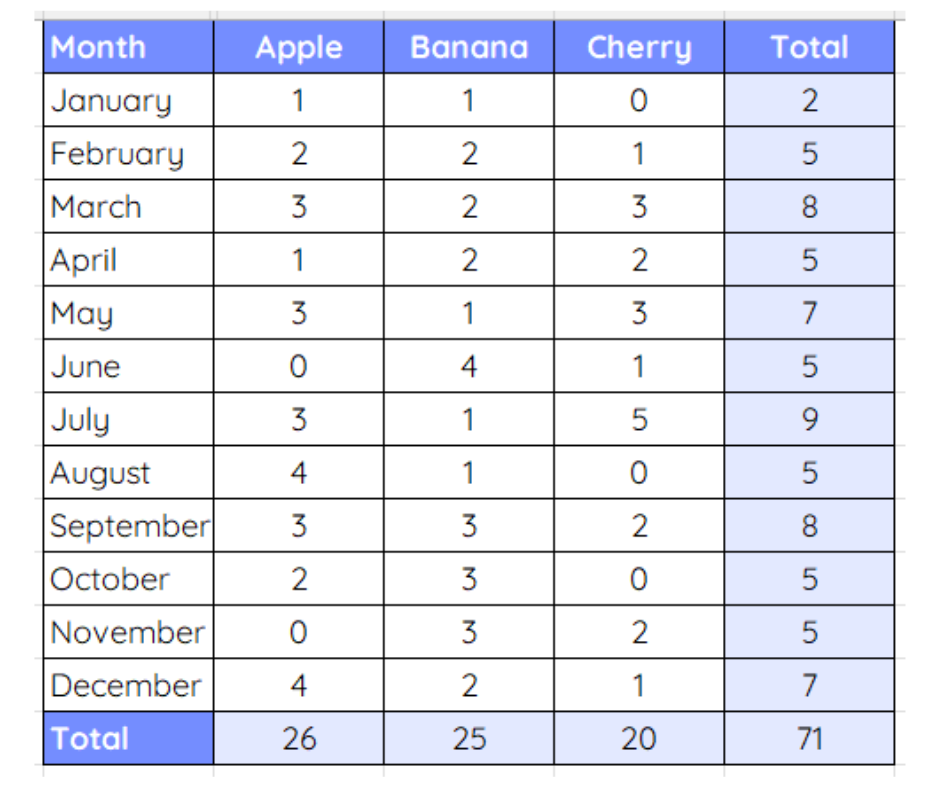
Here’s my summary table:

Notice how I’ve included a column with the start and end date of each month within it. This is going to save a whole lot of time later (and can be hidden when I’m finished) so hear me out!
In cell G2, I’m going to write the following calculation:
=COUNTIFS(A:A,">="&E2,A:A,"<="&F2,B:B,G1)
Here's what it means:
Argument | What does it mean? |
A:A | Range 1 - This is the column in our data that contains the date. It's used twice within the calculation. |
">="&E2 | Criteria 1 - This means "Greater than or equal to" the contents of E2. In our example, this is 01/01/2021. Essentially, it's asking the COUNTIF to look through the data in column A and look for any dates that are "greater than or equal to 01/01/2021". This would be all of the dates if we didn't add a second set of arguments. |
A:A | Range 2 - as before, its the column that contains all the dates. |
"<="&F2 | Criteria 2 - This part asks if any cells in column A are "Less than or equal to" the contents of F2, or the 31/01/3021. |
B:B | Range 3 - We now need to evaluate the actual products brought so this range contains this information. |
G1 | Criteria 3 - G1 contains the word "apple", so is asking the function to look for this word in column B. |
As you can see below, the answer displayed is 1. To sense check this, you’ll see there are only 2 sales in January 2021, 1 for apple and 1 for banana. This matches up nicely!

To complete the table, I’ll need to think carefully about the cell addressing I need to use.
Cell addressing is basically deciding whether you need to fix cell references (absolute) or not (relative), using the dollar sign ($). Think of the dollar ($) as a little dot of glue. If it’s there, cell references stay put, if not they are going to move.
Here is my adjusted calculation:
=COUNTIFS($A:$A,">="&$E2,$A:$A,"<="&$F2,$B:$B,G$1)
As a rule, you are normally always going to need to fix ranges. These are any cell references seen together and separated with a colon (:). There are quite a few in our example, A:A x 2 and B:B so fix these using absolute cell addressing.
Next review the individual cells. These need to be considered more carefully.
E2 - fix the column only, so it becomes $E2.
F2 - as above, fix the column only to make it $F2
G1 - this time fix the row only. Make it G$1.
If you get this right, you are ready to complete the whole of the summary table in a couple of clicks.
Use your fill handle in G2 to complete sales for apple vertically, then drag across to complete horizontally. The video below explains this better so hit play!
You have now created a report that provides you with the total number of items sold, per month.

Why not finish it up by selecting all the blank cells and using the cheeky keyboard shortcut. seen here:
So there you have it. An interesting twist on the COUNTIFS function.

Have you used this method before to create a summary table? Comment below and let me know!
Don't forget you can follow me on Instagram, for daily Microsoft Excel hints and tips!

Yorumlar